GRAPE for time-dependent hamiltonians#
Simulation#
## MAIN.py with time_dep example

import jax
import jax.numpy as jnp
from feedback_grape.grape import (
    optimize_pulse,
    plot_control_amplitudes,
    fidelity,
)
from feedback_grape.utils.solver import sesolve
from feedback_grape.utils.operators import identity, destroy, sigmap, sigmaz
from feedback_grape.utils.tensor import tensor
from feedback_grape.utils.states import basis
# ruff: noqa

N_cav = 10
chi = 0.2385 * (2 * jnp.pi)
mu_qub = 4.0
mu_cav = 8.0
hconj = lambda a: jnp.swapaxes(a.conj(), -1, -2)
time_start = 0.0
time_end = 1.0
time_intervals_num = 5
N_cav = 10
# Eqivalant to delta_ts = jnp.repeat(0.2, time_intervals_num).astype(jnp.float32)
# However, it is implemented in this way to be more general and
# show that these are the differences between the time intervals
t_grid = jnp.linspace(time_start, time_end, time_intervals_num + 1)
delta_ts = t_grid[1:] - t_grid[:-1]
fake_random_key = jax.random.key(seed=0)
e_data = jax.random.uniform(
    fake_random_key, shape=(4, len(delta_ts)), minval=-1, maxval=1
)
e_qub = e_data[0] + 1j * e_data[1]
e_cav = e_data[2] + 1j * e_data[3]


@jax.vmap
def build_ham(e_qub, e_cav):
    """
    Build Hamiltonian for given (complex) e_qub and e_cav
    """

    a = tensor(identity(2), destroy(N_cav))
    adag = hconj(a)
    n_phot = adag @ a
    sigz = tensor(sigmaz(), identity(N_cav))
    sigp = tensor(sigmap(), identity(N_cav))
    one = tensor(identity(2), identity(N_cav))

    H0 = +(chi / 2) * n_phot @ (sigz + one)

    H_ctrl = mu_qub * sigp * e_qub + mu_cav * adag * e_cav
    H_ctrl += hconj(H_ctrl)
    # You just pass an array of the Hamiltonian matrices "Hs" corresponding to the time
    # intervals "delta_ts" (that is, "Hs" is a 3D array).
    return H0, H_ctrl


H0, H_ctrl = build_ham(e_qub, e_cav)


# Representation for time dependent Hamiltonian
def solve(Hs, delta_ts):
    """
    Find evolution operator for piecewise Hs on time intervals delts_ts
    """
    for i, (H, delta_t) in enumerate(zip(Hs, delta_ts)):
        U_intv = jax.scipy.linalg.expm(-1j * H * delta_t)
        U = U_intv if i == 0 else U_intv @ U
    return U


U = solve(H0 + H_ctrl, delta_ts)
psi0 = tensor(basis(2), basis(N_cav))
global psi_target_qt
psi_target_qt = psi_target = U @ psi0


def build_grape_format_ham():
    """
    Build Hamiltonian for given (complex) e_qub and e_cav
    """

    a = tensor(identity(2), destroy(N_cav))
    adag = hconj(a)
    n_phot = adag @ a
    sigz = tensor(sigmaz(), identity(N_cav))
    sigp = tensor(sigmap(), identity(N_cav))
    one = tensor(identity(2), identity(N_cav))

    H0 = +(chi / 2) * n_phot @ (sigz + one)
    H_ctrl_qub = mu_qub * sigp
    H_ctrl_qub_dag = hconj(H_ctrl_qub)
    H_ctrl_cav = mu_cav * adag
    H_ctrl_cav_dag = hconj(H_ctrl_cav)

    H_ctrl = [H_ctrl_qub, H_ctrl_qub_dag, H_ctrl_cav, H_ctrl_cav_dag]

    return H0, H_ctrl


def test_time_dep(optimizer="adam"):
    H0_grape, H_ctrl_grape = build_grape_format_ham()

    res = optimize_pulse(
        H0_grape,
        H_ctrl_grape,
        psi0,
        psi_target,
        int(
            (time_end - time_start) / delta_ts[0]
        ),  # Ensure this is an integer
        time_end - time_start,
        max_iter=10000,
        # when you decrease convergence threshold, it is more accurate
        convergence_threshold=1e-3,
        learning_rate=1e-2,
        evo_type="state",
        optimizer=optimizer,
    )
    return res
res_fg = test_time_dep("l-bfgs")
print(res_fg.final_fidelity)
print(res_fg.iterations)
0.9977032330308184
152
time_start = 0.0
time_end = 1.0
time_intervals_num = 5
t_grid = jnp.linspace(time_start, time_end, time_intervals_num)
H_labels = [r'$u_1$', r'$u_2$', r'$u_3$', r'$u_4$', r'$u_5$']
t_grid.shape
(5,)
res_fg.control_amplitudes.shape
(5, 4)
plot_control_amplitudes(t_grid, res_fg.control_amplitudes, labels=H_labels)
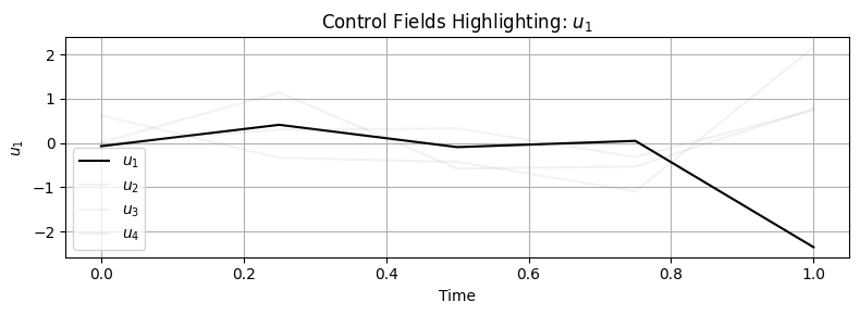
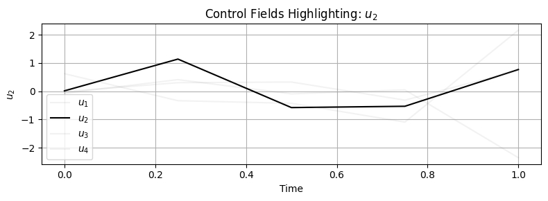
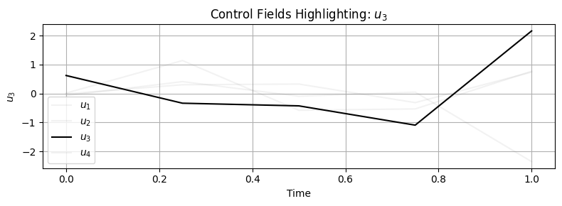
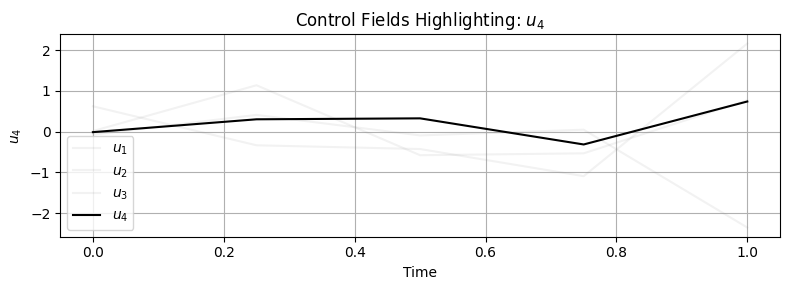
res_fg.control_amplitudes
Array([[-0.07147105,  0.01470273,  0.6226829 , -0.01167848],
       [ 0.41113622,  1.13837515, -0.33436464,  0.30311274],
       [-0.09246789, -0.57771355, -0.4260761 ,  0.32651927],
       [ 0.04823766, -0.53138383, -1.09182372, -0.31420846],
       [-2.35143086,  0.76905461,  2.16170908,  0.73981248]],      dtype=float64)
Example of user trying to construct his time dependent Hamiltonian from extracted amplitudes and then get the final operator#
Define the time grid (same as defined)#
time_start = 0.0
time_end = 1.0
time_intervals_num = 5
N_cav = 10
# Eqivalant to delta_ts = jnp.repeat(0.2, time_intervals_num).astype(jnp.float32)
# However, it is implemented in this way to be more general and
# show that these are the differences between the time intervals
t_grid = jnp.linspace(time_start, time_end, time_intervals_num + 1)
delta_ts = t_grid[1:] - t_grid[:-1]
Build the Hamiltonian#
def build_ham_reconstructed(u1, u2, u3, u4):
"""
Build Hamiltonian for given (complex) e_qub and e_cav
"""
a = tensor(identity(2), destroy(N_cav))
adag = hconj(a)
n_phot = adag @ a
sigz = tensor(sigmaz(), identity(N_cav))
sigp = tensor(sigmap(), identity(N_cav))
one = tensor(identity(2), identity(N_cav))
H0 = +(chi / 2) * n_phot @ (sigz + one)
H_ctrl_qub = mu_qub * sigp
H_ctrl_qub_dag = hconj(H_ctrl_qub)
H_ctrl_cav = mu_cav * adag
H_ctrl_cav_dag = hconj(H_ctrl_cav)
# Apply control amplitudes
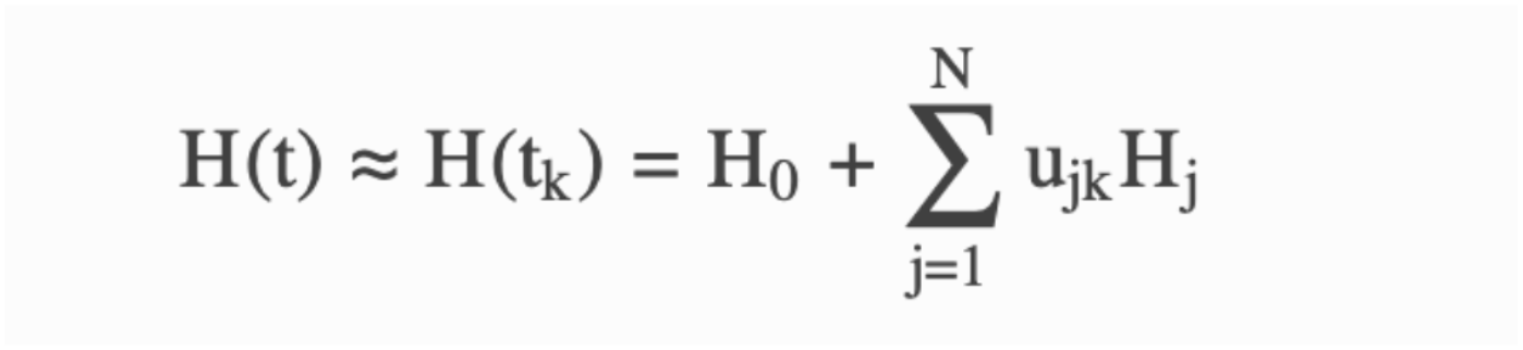
H_ctrl = (
u1 * H_ctrl_qub
+ u2 * H_ctrl_qub_dag
+ u3 * H_ctrl_cav
+ u4 * H_ctrl_cav_dag
)
H = H0 + H_ctrl
return H
u1 = res_fg.control_amplitudes[:, 0]
u2 = res_fg.control_amplitudes[:, 1]
u3 = res_fg.control_amplitudes[:, 2]
u4 = res_fg.control_amplitudes[:, 3]
u1
Array([-0.07147105, 0.41113622, -0.09246789, 0.04823766, -2.35143086], dtype=float64)
Construct the Hamiltonian for each time step#
H_total = jnp.array(
    [
        build_ham_reconstructed(u1[i], u2[i], u3[i], u4[i])
        for i in range(len(u1))
    ]
)
H_total
Array([[[  0.        +0.j,  -0.09342782+0.j,   0.        +0.j, ...,
           0.        +0.j,   0.        +0.j,   0.        +0.j],
        [  4.98146318+0.j,   1.4985397 +0.j,  -0.13212689+0.j, ...,
           0.        +0.j,   0.        +0.j,   0.        +0.j],
        [  0.        +0.j,   7.04485279+0.j,   2.99707939+0.j, ...,
           0.        +0.j,   0.        +0.j,   0.        +0.j],
        ...,
        [  0.        +0.j,   0.        +0.j,   0.        +0.j, ...,
           0.        +0.j,  -0.26425378+0.j,   0.        +0.j],
        [  0.        +0.j,   0.        +0.j,   0.        +0.j, ...,
          14.08970559+0.j,   0.        +0.j,  -0.28028346+0.j],
        [  0.        +0.j,   0.        +0.j,   0.        +0.j, ...,
           0.        +0.j,  14.94438955+0.j,   0.        +0.j]],

       [[  0.        +0.j,   2.42490192+0.j,   0.        +0.j, ...,
           0.        +0.j,   0.        +0.j,   0.        +0.j],
        [ -2.67491714+0.j,   1.4985397 +0.j,   3.42932918+0.j, ...,
           0.        +0.j,   0.        +0.j,   0.        +0.j],
        [  0.        +0.j,  -3.7829041 +0.j,   2.99707939+0.j, ...,
           0.        +0.j,   0.        +0.j,   0.        +0.j],
        ...,
        [  0.        +0.j,   0.        +0.j,   0.        +0.j, ...,
           0.        +0.j,   6.85865835+0.j,   0.        +0.j],
        [  0.        +0.j,   0.        +0.j,   0.        +0.j, ...,
          -7.56580821+0.j,   0.        +0.j,   7.27470575+0.j],
        [  0.        +0.j,   0.        +0.j,   0.        +0.j, ...,
           0.        +0.j,  -8.02475143+0.j,   0.        +0.j]],

       [[  0.        +0.j,   2.61215413+0.j,   0.        +0.j, ...,
           0.        +0.j,   0.        +0.j,   0.        +0.j],
        [ -3.4086088 +0.j,   1.4985397 +0.j,   3.69414379+0.j, ...,
           0.        +0.j,   0.        +0.j,   0.        +0.j],
        [  0.        +0.j,  -4.82050079+0.j,   2.99707939+0.j, ...,
           0.        +0.j,   0.        +0.j,   0.        +0.j],
        ...,
        [  0.        +0.j,   0.        +0.j,   0.        +0.j, ...,
           0.        +0.j,   7.38828759+0.j,   0.        +0.j],
        [  0.        +0.j,   0.        +0.j,   0.        +0.j, ...,
          -9.64100159+0.j,   0.        +0.j,   7.83646238+0.j],
        [  0.        +0.j,   0.        +0.j,   0.        +0.j, ...,
           0.        +0.j, -10.2258264 +0.j,   0.        +0.j]],

       [[  0.        +0.j,  -2.51366765+0.j,   0.        +0.j, ...,
           0.        +0.j,   0.        +0.j,   0.        +0.j],
        [ -8.73458974+0.j,   1.4985397 +0.j,  -3.55486289+0.j, ...,
           0.        +0.j,   0.        +0.j,   0.        +0.j],
        [  0.        +0.j, -12.35257527+0.j,   2.99707939+0.j, ...,
           0.        +0.j,   0.        +0.j,   0.        +0.j],
        ...,
        [  0.        +0.j,   0.        +0.j,   0.        +0.j, ...,
           0.        +0.j,  -7.10972577+0.j,   0.        +0.j],
        [  0.        +0.j,   0.        +0.j,   0.        +0.j, ...,
         -24.70515053+0.j,   0.        +0.j,  -7.54100296+0.j],
        [  0.        +0.j,   0.        +0.j,   0.        +0.j, ...,
           0.        +0.j, -26.20376921+0.j,   0.        +0.j]],

       [[  0.        +0.j,   5.91849981+0.j,   0.        +0.j, ...,
           0.        +0.j,   0.        +0.j,   0.        +0.j],
        [ 17.29367265+0.j,   1.4985397 +0.j,   8.3700227 +0.j, ...,
           0.        +0.j,   0.        +0.j,   0.        +0.j],
        [  0.        +0.j,  24.4569464 +0.j,   2.99707939+0.j, ...,
           0.        +0.j,   0.        +0.j,   0.        +0.j],
        ...,
        [  0.        +0.j,   0.        +0.j,   0.        +0.j, ...,
           0.        +0.j,  16.7400454 +0.j,   0.        +0.j],
        [  0.        +0.j,   0.        +0.j,   0.        +0.j, ...,
          48.9138928 +0.j,   0.        +0.j,  17.75549943+0.j],
        [  0.        +0.j,   0.        +0.j,   0.        +0.j, ...,
           0.        +0.j,  51.88101794+0.j,   0.        +0.j]]],      dtype=complex128)
H_total.shape
(5, 20, 20)
Solve the Schrödinger Equation#
psi0_fg = tensor(basis(2), basis(N_cav))
psi_fg = sesolve(H_total, psi0_fg, delta_ts, evo_type="state")
Calculate fidelity with target#
print(fidelity(C_target=psi_target, U_final=psi_fg, evo_type="state"))
0.9977032330308189